Get started with NCA
There are three ways to get started with NCA and to check whether your data may contain a necessary condition.
1. Visual inspection of scatter plot
Checking the XY-scatter plot of your observations is the simplest way to evaluate whether your data may contain a necessary condition. When the values of the condition X increase horizontally to the right, and the values of the outcome Y increase vertically upwards, an empty space (spaces without observations) in the upper-left corner of the scatter plot may indicate that you have found a necessary condition.
2. NCA Calculator
Using the NCA Calculator on this website is another quick way to run a quantitative NCA analysis. If you upload a CSV file that contains your data (X = condition, Y = Outcome), the NCA calculator will run a simple NCA. The NCA calculator gives the effect size of the necessity of X for Y. When the effect size is greater than 0 (and in particular when it is above 0.1) you may have found a necessary condition.
3. NCA Software
You can use the NCA Software for R to run a complete NCA analysis. R is an open source programming language that is increasingly used for data analysis in different scientific fields, including the social sciences. It contains many statistical, mathematical and graphical functions that are also part of commercial statistical software such as SPSS and SAS. Additionally, R can run specific user-defined functions (“packages”). One such package is NCA. Only some basic knowledge about R is needed to run NCA with R. A Quick Start Guide is available (also here) to help a novice user without knowledge of R or NCA to perform an NCA analysis with R within 15 minutes.
Example
The example shows how NCA can be used to build or test necessity theory. The example has two parts: the first part shows a bivariate NCA (one X=condition, one Y=outcome), and the second part shows a multiple NCA (more than one X, one Y).
Bivariate NCA
Suppose that a researcher explores or tests a necessity theory about the relationship between a country's cultural values and a country's innovation performance, represented by the following necessity hypothesis:
H1 Individualism is necessary for Innovation performance.
Note that usual hypotheses such as “If individualism is higher, then (it is likely that) Innovation performance is higher” are sufficiency hypotheses. Note also that commonly used general hypotheses (“Individualism has an effect on Innovation performance”, “Individualism is associated with Innovation performance”, “Individualism affects Innovation performance”, etc.) are interpreted as sufficiency hypotheses, although they could also be interpreted and specified as necessity hypotheses.
Suppose that the sample consists of 28 countries (for which data are available for the independent and dependent variables).
Measurement
Suppose that the scores of Individualism are obtained from Hofstede's (1980) cultural dimensions, and the scores of a country's innovation performance from Gans and Stern's (2003) innovation index, and that these scores are valid and reliable.
Data analysis with NCA
In six steps (Dul, 2016, Tables 3 and 4) a necessity hypothesis can be explored or tested with NCA:
Step 1: Make the scatter plot.
Make a XY scatter plot for (X=Individualism, Y=Innovation performance) with X axis ‘‘horizontal’’ and the Y axis ‘‘vertical’’ and values increase ‘‘to the right’’ and ‘‘upward.’’ The example scatter plot is displayed below.
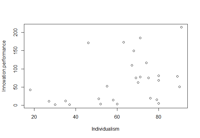
Each dot represents a case (country). The Individualism scores (X) range from 18 to 91, and the Innovation performance scores (Y) from 1.2 to 214.4.
Step 2: Identify the empty space
Visually inspect if the upper left corner of the scatter plot is empty. Consider to allow some exceptions (e.g., 5% of all observations) in the ‘‘empty space.’’ If there is no ‘‘empty space,’’ (hence the upper left corner has observations) a necessary condition is not present, and the necessity hypothesis can be rejected. In the example scatter plot there is an empty area in the upper-left corner, indicating that there may be a necessary condition.
Step 3: Draw the ceiling line
Select one of the two ceiling line techniques:
- CE-FDH (red): Ceiling Envelopment with Free Disposal Hull (CE-FDH). This is a piecewise linear function that can be used when the data are discrete (few possible levels of the X variable).
- CR-FDH (orange): Ceiling Regression with Free Disposal Hull (CE-FDH). This is a straight line that can be used when the data and underlying phenomenon is (approximately) continuous (large number of possible levels of the X variable).
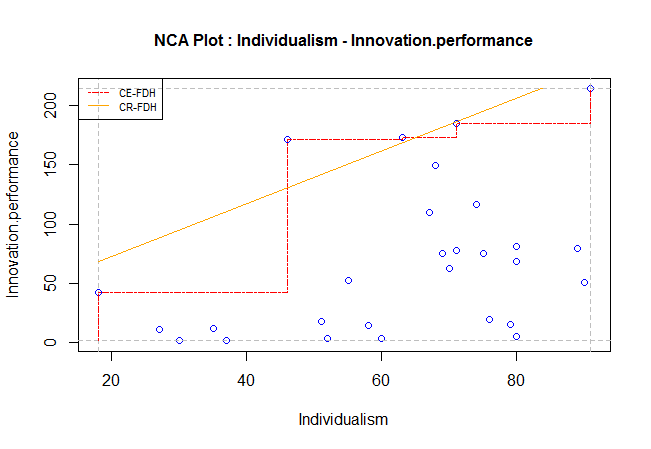
The CE-FDH ceiling line is the red dashed line, which can be manually drawn by starting at the XY-point corresponding to the lowest observed X-value and the lowest observed Y value (0,0), then moving vertically upward to the observation with the largest Y for the lowest X (there can be more than one observation with the same X-value, particularly for discrete variables), then moving horizontally to the right until the point with an observation on or above this horizontal line (discard observations below this line). Afterwards move vertically upward to the observation with the largest Y for this X (again there can be more than one observations with the same X value, particularly for discrete variables), and continue this process until the final point.
The CR-FDH ceiling line is the orange line, which is the ordinary least squares trend line trough the upper-left edges ("north-west" corners) of the CE-FDH step function. CR-FDH smooths CE-FDH.
The NCA Software or the NCA Calculator can be used to draw these lines in the scatter plot. Both tools include this example.
Step 4: Quantify the NCA parameters
In this example we calculated NCA parameters for the CR-FDH ceiling line. The parameters can be calculated with the NCA Software.
Scope: the area where observations can be expected given the highest and lowest X and Y values: Multiply the highest minus the lowest X values, with the highest minus the lowest Y values. For the example the value of the scope is (91 - 18) x (214.4 - 1.2) = 15564
Ceiling zone: the size of the ‘‘empty space.’’ For the example this is the area above the orange CR-FDH ceiling line, which is 4773.
Effect size (d): Divide Ceiling zone by Scope. For the example the value of the effect size is 0.307. The effect size is one of the most important NCA parameters. It represents the extent to which the condition constrains the outcome.
Accuracy: the number of observations that are not in the ‘‘empty space,’’ divided by the total number of observations, multiplied by 100%. For the example the value of accuracy is 92.9%, because two observations are above the orange ceiling line.
Two more advanced NCA parameters are condition inefficiency and outcome inefficiency. Condition inefficiency is the percentage of the range of the condition where the condition is not necessary for the outcome. For the example the value of condition inefficiency is 10.3%, indicating that for only about 10% of the range of X (the highest levels), the condition does not constrain the outcome (hence, for almost 90% of the X-range, X constrains Y). Outcome inefficiency is the percentage of the range of the outcome where the condition is not necessary for the outcome. For the example the value of outcome inefficiency is 31.6 %, indicating that for about 1/3rd of the range of Y (the lower levels), the outcome is not constrained by the condition (hence, for more than 2/3rd of the Y-range, Y is constrained by X).
Step 5: Evaluate effect size and accuracy
Evaluate if the effect size (d) is theoretically or practically meaningful in the current context. Consider using the general benchmark 0 < d < 0.1 ‘‘small effect,’’ 0.1 ≤ d < 0.3 ‘‘medium effect,’’ 0.3 ≤ d <0.5 ‘‘large effect,’’ and d ≥ 0.5 ‘‘very large effect.’’ Compare the accuracy with the benchmark of 95%. If effect size and accuracy are considered large enough, continue with Step 6. In the example the necessity effect size can be considered as meaningful with a medium effect size. The accuracy is somewhat low due to the small number of observations with 2 observations are above the ceiling line.
Step 6: Formulate the necessary condition
If the researcher concludes from Step 5 that the necessary condition is present in the current sample, the necessary condition can be formulated in general terms (in kind) as ‘‘Individualism is necessary for Innovation performance’’. Additionally the necessary condition can be formulated more detailed (in degree) by formulating the ceiling line Yc = 2.2Xc + 28.4 indicating which minimum level of Xc is necessary for which level of Yc. The slope and intercept of the ceiling line are calculated with the NCA Software.
Warning: just like any other research approach and data analysis technique NCA has several limitations.
Multiple NCA
In multiple NCA there is more than one potential necessary condition (X1, X2, …) and one outcome (Y). We can extend the bivariate example by adding another potential necessary condition for Innovation performance, for example Risk taking. Then there are two necessity hypotheses:
H1 Individualism is necessary for Innovation performance.
H2 Risk taking is necessary for Innovation performance.
For a multiple NCA, first the bivariate analyses is made for each condition separately, because a necessary condition operates independently from the rest of the causal structure. Hence steps 1-6 are repeated for Risk taking. It turns out, when using the NCA Software or NCA Calculator, that Risk taking is also necessary for Innovation performance with effect size 0.282, which can be considered as a medium effect size.
A multiple NCA with two necessary conditions is a necessary AND configuration, which can be represented by a ceiling surface.
For the interpretation of the multiple NCA the bottleneck table can be helpful. The bottleneck table is a tabular representation of the ceiling lines of one or multiple necessary conditions. It shows the required necessary level of the conditions (X1=Individualism, X2=Risk taking) for a given level of the outcome (Y=Innovation performance), see below.
Y X1 X2
0 NN NN
10 NN NN
20 NN NN
30 NN 8.0
40 11.0 17.1
50 24.1 26.2
60 37.2 35.2
70 50.3 44.3
80 63.4 53.4
90 76.5 62.4
100 89.6 71.5
The level of the conditions and outcome are expressed as percentage of the range: 0 is the minimum observed value, 100 is the maximum observed value, and 50 is the value in between these two values. The bottleneck table for the example shows that for a level of the outcome Y=20 no minimum value of Individualism (X1), and no minimum value of Risk taking (X2) are required for that ourcome to occur (NN= Not Necessary). However, for Y=30, a minimum value of 8.0 is required for Risk taking, and for Y=40 a minimum value of 11.0 is required for Individualism, and a minimum value of 17.1 is required for Risk taking. For Y=100 (maximum Innovation performance), a minimum value of 89.6 for Individualism, and of 71.5 for Risk taking are required. If in practice one of these minimum levels is not achieved, the outcome Y=100 will not occur. Hence, each condition can be a bottleneck.