Workbook 2: 'Differences between independent groups - binary data.xlsx'
The workbooks and a pdf-version of this user manual can be downloaded from here.
Input sheet
The required input for this workbook is not a point estimate with a standard error (such as in Workbook 1). Instead, the user must enter either the number of cases with either outcome in each group (see cells a, b, c, and d in the two-by-two table on the right side of Figure 45). Or any other combination of information that makes it possible to calculate these four numbers. In practice this means that the user must fill at least four of the six cells in this two-by-two table. Each of the rows in Figure 45 represents a study with sufficient information according to this principle.
It is a unique feature of this workbook that an effect size (e.g., an odds ratio by) can be converted into another one (e.g., a risk difference). It is not possible to insert any one of these effect sizes directly in this workbook, because this conversion is not possible without the full information from the 2x2 table.
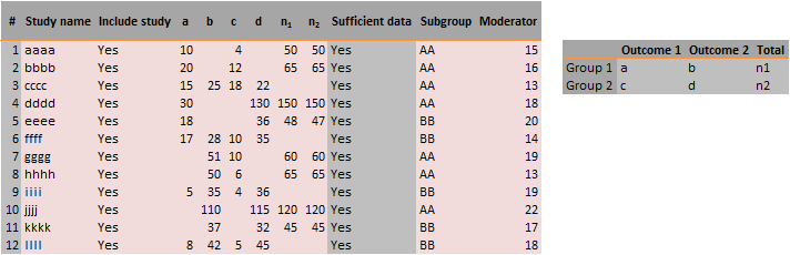
Figure 45: Input sheet of Workbook 2 ‘Differences between independent groups - binary data.xlsx’
Forest Plot sheet
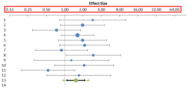
A unique feature of this workbook is an additional forest plot that presents the effect sizes on a logarithmic scale, see red rectangle in Figure 46 for an example. Note that the lowest value on the x-axis shows ‘0.13’ instead of ‘0.125’ because of rounding. This makes it easier to interpret the results of the meta-analysis when the odds ratio or risk ratio is selected as the effect size measure. It is recommended to always use the logarithmic forest plot for the presentation of a meta-analysis of odds ratios or risk ratios and to use the ‘normal’ forest plot for risk differences only.
Weighting methods
The user can choose between three weighting methods: the standard inverse variance method, the Mantel-Haenszel method (Mantel & Haenszel, 1959) or the Peto-Odds method (Peto et al., 1977, p. 31).
Meta-analysis model and presentation effect size
From a statistical perspective, meta-analysing (Log) Odds Ratios is preferable because the Odds Ratio is less prone to heterogeneity (compared to Risk Difference in particular). On the down side, however, the Odds Ratio is rather hard to interpret.
In this workbook the user can select an effect size for the meta-analysis model (i.e. the effect size measure used in the calculations) and another one for presentation in the forest plot. All calculations can be inspected on the Calculations sheet. Note that conversion is performed only from Odds Ratio to Risk Ratio or Risk Difference (‘downstream’), not the other way around, because there is no use for the opposite direction.
For the inverse variance weighting method, the user can also choose between using the Odds Ratio, Risk Ratio and Risk Difference (for both the model and the presentation). If you choose the Odds Ratio or Risk Ratio for the model, the meta-analysis will actually be run in Log Odds Ratio and Log Risk Ratio respectively. For the Peto weighting method, a slightly different Odds Ratio is available, called the Peto Odds Ratio, whereas all other options are available as well.
Note that a weighting method must be chosen before the effect size measure, because not all options (for effect size measure) are available for all weighting methods. The user is informed about the ‘validity’ (‘Yes’ or ‘No’) of a combination that is selected in the ‘Valid options chosen’ row (see Figure 47).
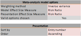
Figure 47: Example of additional selection options on the Forest Plot sheet of Workbook 2 ‘Differences between independent groups - binary data.xlsx’
Statistical procedures
Some non-standard solutions are used in this workbook for conversion of statistics for Odds Ratio to statistics for Risk Difference, particularly for the standard error (which affects the calculation of the confidence and prediction interval). The basic premise of this procedure is that the statistical significance of the various statistics is equal. See the working paper on the website for this method by Van Rhee & Suurmond (2015).
Note that not all the heterogeneity measures are scale-free and that they are based on the effect size measure of the model, not the effect size measure of the presentation. This means that the scale of the heterogeneity measures depends on the choice of the effect size measure in the model.
Subgroup Analysis sheet
In the Subgroup Analysis it is not possible to make separate choices of effect size measure for the model and the presentation.
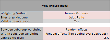
Figure 48: Options for Subgroup Analysis in Workbook 2 ‘Differences between independent groups - binary data.xlsx’
Moderator Analysis sheet
The moderator regression for binary data can be run in Log Odds Ratio, Log Risk Ratio or Risk Difference. The logarithmic values of the Odds Ratio and Risk Ratio are used instead of the ‘normal’ values because they tend to normality faster (see Figure 49).
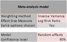
Figure 49: Options for Moderator Analysis in Workbook 2 ‘Differences between independent groups - binary data.xlsx’
Publication Bias Analysis sheet
Procedures for assessing publication bias for binary data can be run in Log Odds Ratio, Log Risk Ratio or Risk Difference (see Figure 50).
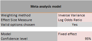
Figure 50: Options for Publication Bias Analysis in Workbook 2 ‘Differences between independent groups - binary data.xlsx’
L’Abbé plot
One additional plot is provided for binary data, the L’Abbé plot (L'Abbé, Detsky, & O'Rourke, 1987) (see Figure 51). This plot gives the Group 2 (e.g., control) risk on the x-axis and the Group 1 (e.g., treatment) risk on the y-axis. A reference line of zero effect (the diagonal) is provided in red along with a blue dotted line that gives the ratio between the risks of group 2 and group 1 (the combined Risk Ratio). The size of the point estimates (blue dots) corresponds to the study weights. The study weights depend on the chosen model (fixed effect versus random effects) and on the chosen weighting method.
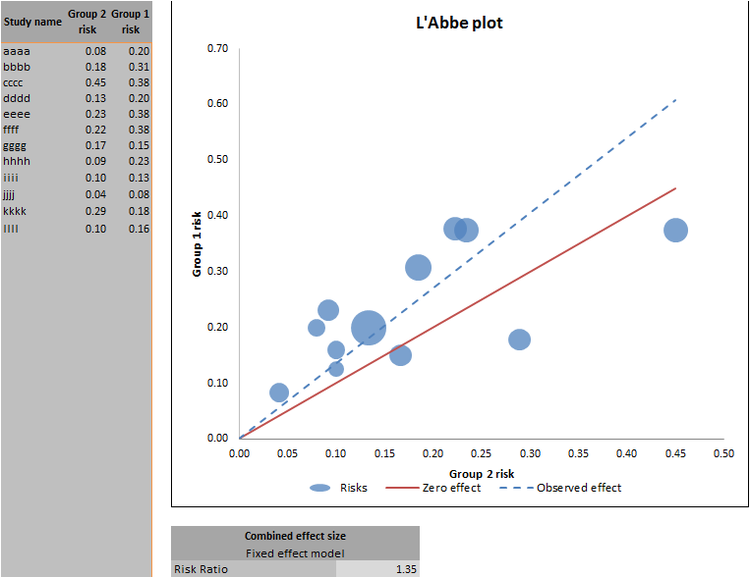
Figure 51: L’Abbé Plot on the Publication Bias Analysis sheet of Workbook 2 ‘Differences between independent groups - binary data.xlsx’
Calculations sheet
The calculations sheet for binary data begins with a repetition of the cell counts and the “Add 0.5” asks whether any of the cells has a count of zero, in which case .5 should be added to all the cell counts because the effect sizes are not calculable otherwise. In this tab, you will see additional columns with log effect sizes for calculation purposes. Two additional headers (and thus chapters of the tab) are provided: ‘Effect Sizes’ and ‘Weighting Methods’. In Effect Sizes, four parts describing the calculations for different effect sizes are given: odds ratio, Peto odds ratio, risk difference and risk ratio (see Figure 52 for an example). In Weighting Methods the three weighting methods are given (Inverse Variance, Mantel-Haenszel and Peto) (see Figure 53 for an example) along with some information for the conversion of one effect size measure into the other (see Figure 54 for an example).
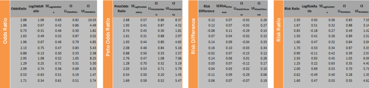
Figure 52 Example of Effect Sizes part of Calculations tab of Workbook 2 ‘Differences between independent groups - binary data.xlsx’

Figure 53 Example of Weighting Method part of Calculations tab of Workbook 2 ‘Differences between independent groups - binary data.xlsx’
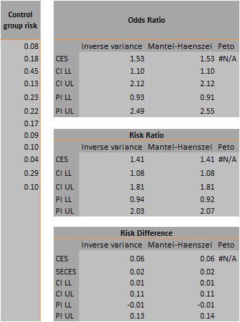
Figure 54: Example of Conversion to Other Effect Size Measures part of Calculations tab of Workbook 2 ‘Differences between independent groups - binary data.xlsx’
References
L'Abbé, K. A., Detsky, A. S., & O'Rourke, K. (1987). Meta-analysis in clinical research. Annals of Internal Medicine, 107(2), 224-233. dx.doi.org/10.7326/0003-4819-108-1-158_2
Mantel, N., & Haenszel, W. (1959). Statistical aspects of the analysis of data from retrospective studies of disease. Journal of the National Cancer Institute, 22(4), 719-748. https://doi.org/10.1093/jnci/22.4.719
Peto, R., Pike, M. C., Armitage, P., Breslow, N. E., Cox, D. R., Howard, S. V., . . . Smith, P. G. (1977). Design and analysis of randomized clinical trials requiring prolonged observation of each patient. II. Analysis and examples. British Journal of Cancer, 35(1), 1-39. dx.doi.org/10.1038/bjc.1977.1
Van Rhee, H. J., & Suurmond, R. (2015). Working paper: Meta-analyze dichotomous data: Do the calculations with log odds ratios and report risk ratios or risk differences. Rotterdam, The Netherlands: Erasmus Rotterdam Institute of Management. www.erim.eur.nl/research-support/meta-essentials/download