Subgroup Analysis sheet
Refer to the Subgroup Analysis page for details on how to interpret.
The workbooks and a pdf-version of this user manual can be downloaded from here.
When the user has entered a category in the ‘Subgroup’ column of the Input sheet, then the Subgroup Analysis sheet will present meta-analytic results for each subgroup separately. For instance, if the user has coded the origin of the data used in a study as either ‘USA’ or ‘Non-USA’, this sheet will give a combined effect size for the ‘USA’ studies and another combined effect size for the ‘Non-USA’ studies, as well as an combined effect size for all included studies. You can access the sheet by clicking on the regarding tab, as shown in Figure 8.

Figure 8: The tab to access the Subgroup Analysis sheet of Meta-Essentials
The left side of this sheet is similar to the left side of the Forest Plot sheet (see Figure 9). For the sake of clarity we make us of a feature of Microsoft Excel that offers the opportunity to ‘hide’ certain columns. These parts can be accessed by clicking the plus sign at the top of the column (see Figure 10). When the first plus is clicked, a table appears with individual study results, combined effect sizes per subgroup and the overall combined effect size (see Figure 11).
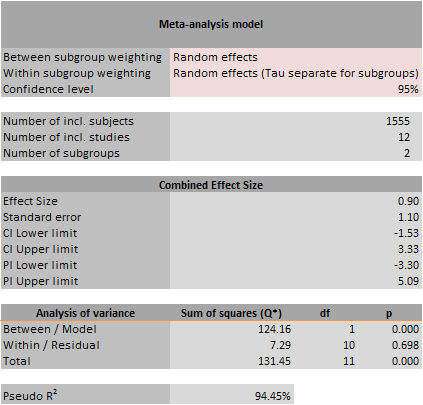
Figure 9: Example of the left part of the Subgroup Analysis sheet
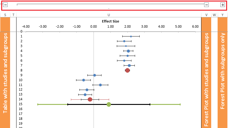
Figure 10: Example of plus signs in the Subgroup Analysis sheet that can be clicked to ‘unhide’ a set of columns
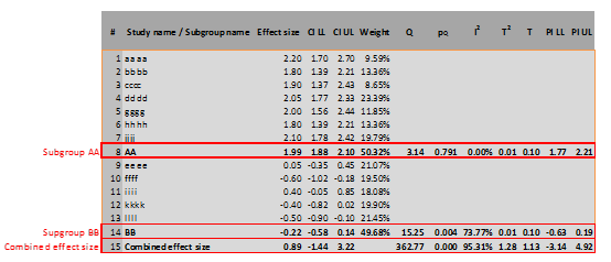
Figure 11: Example of ‘Table with studies and subgroups’ of the Subgroup Analysis sheet
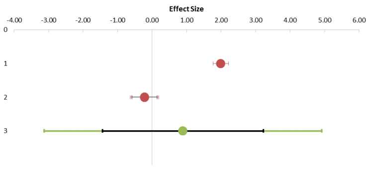
Furthermore, two types of forest plots are available: one with studies, subgroups and combined effect (see Figure 12) and one with subgroup and combined effects only, which enhances the comparison of subgroups (see Figure 13). In these plots, blue dots represent individual studies, red dots represent subgroups, and the green dot represents the combined effect size. Also the prediction intervals are shown for the subgroups and combined effect size in their respective colours, whereas the confidence interval is shown in black. Note that because the confidence interval of the first subgroup in the example of Figures 9 and 10 is so small that it disappears almost entirely behind the red dot.
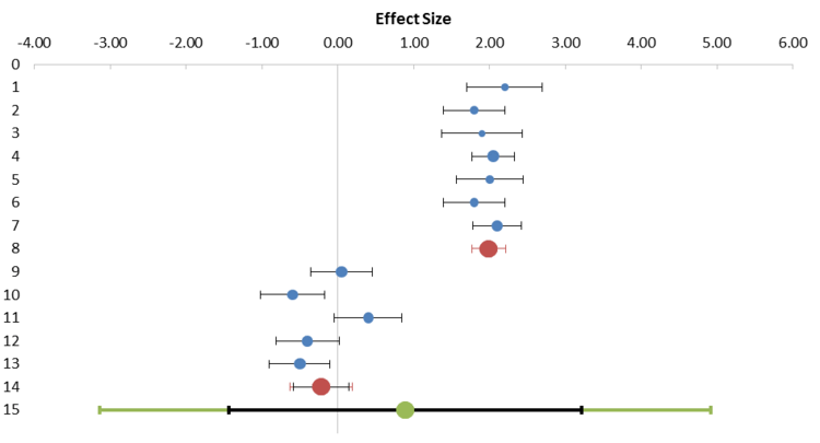
Figure 12: Example of ‘Forest plot with studies and subgroups’ part of the Subgroup Analysis sheet
Options
The user must choose how to distribute weights to studies between subgroups and within subgroups (see the red rectangle labelled ‘Choose options here’ in Figure 9). For the ‘Between subgroup weighting’ the user can choose from a ‘fixed effect’ and ‘random effects’ (default) model. For the ‘Within subgroup weighting’, the user can choose between ‘fixed effect’, ‘random effects (Tau separate for subgroups)’ (default), and ‘random effects (Tau pooled over subgroups)’ models. If the latter option is selected, the variance components (Tau) of each subgroup will be pooled (averaged) and used for every subgroup. Note that these defaults are not always appropriate to use. Theory will have to tell which option to use; in general, using pooled variance components is more appropriate when you have very few studies included in your meta-analysis or in any particular subgroup (Borenstein, Hedges, & Higgins, 2009, pp. 149 ff).
Analysis of variance
This table provides statistics for an analysis of variance based on sums of squares (Q). The table automatically provides these sums of squares based on the model specification (fixed effect or random effects within the subgroups), hence, based on actual weights of the individual studies. Under the fixed effect model, Q (no asterisk) can be used to assess the heterogeneity in the given group, as in a regular meta-analysis. However, under the random effects model within subgroups, Q* can only be used to partition the total variance in within (or residual) and between (or model) variance—and not to test the homogeneity of effects. The amount of variance explained by the model (Q/Q* between) can be used to test whether the combined effect sizes of the subgroups are equal.
References
Borenstein, M. (2009). Effect sizes for continuous data. In H. Cooper, L. V. Hedges & J. C. Valentine (Eds.), The handbook of research synthesis and meta-analysis (Second Ed.) (pp. 221-235). New York, NY: Russell Sage Foundation. www.worldcat.org/oclc/264670503
Higgins, J. P. T., Thompson, S. G., Deeks, J.J., & Altman, D.G. (2003) Measuring inconsistency in meta-analyses. British Medical Journal, 327(7414), 557-560. dx.doi.org/10.1136/bmj.327.7414.557